from matplotlib import pyplot as plt
import numpy as np
import pandas as pd
import geopandas as gpd
np.random.seed(42)
%matplotlib inline

plt.rcParams['figure.figsize'] = (10,6)

Lecture 10B: Clustering Analysis in Python

Nov 5, 2020

Housekeeping

• Assignment #5 (optional) by 5pm on Saturday (2-day extension)
• Assignment #6 (optional) assigned today and due in two weeks (11/19)
  • Covers urban street networks and osmnx
  • Plotting a folium heatmap of a dataset of your choosing — similar to building permit example from last lecture
• Remember, you have to do one of homeworks #4, #5, or #6

Last lecture (10A)

• Making a Folium Choropleth the "hard way" — using folium.GeoJson()
• Folium heatmap of new construction permits in Philadelphia
• Introduction to clustering with scikit-learn
• K-means algorithm for non-spatial clustering

Today

• Exercise on non-spatial clustering with k-means: Airbnb data in Philly neighborhoods
• Spatial clustering with the DBSCAN algorithm
• Exercise on spatial clustering of NYC taxi trips

Part 1: Non-spatial clustering

The goal

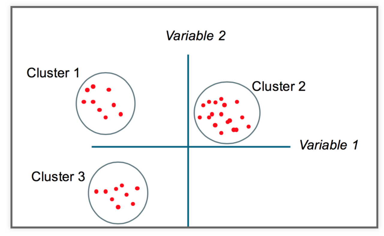
Partition a dataset into groups that have a similar set of attributes, or features, within the group and a dissimilar set of features between groups.

Minimize the intra-cluster variance and maximize the inter-cluster variance of features.

Some intuition

K-Means clustering

• Simple but robust clustering algorithm
• Widely used
• Important: user must specify the number of clusters
• Cannot be used to find density-based clusters

Example: Clustering countries by health and income

• Health expectancy in years vs. GDP per capita and population for 187 countries (as of 2015)
• Data from Gapminder

import altair as alt
from vega_datasets import data as vega_data

Read the data from a URL:

gapminder = pd.read_csv(vega_data.gapminder_health_income.url)
gapminder.head()

	country	income	health	population
0	Afghanistan	1925	57.63	32526562
1	Albania	10620	76.00	2896679
2	Algeria	13434	76.50	39666519
3	Andorra	46577	84.10	70473
4	Angola	7615	61.00	25021974

K-Means with scikit-learn

from sklearn.cluster import KMeans

kmeans = KMeans(n_clusters=5)

Normalizing features with the pre-processing module

• Scikit-learn has a utility to normalize features with an average of zero and a variance of 1
• Use the StandardScaler class

from sklearn.preprocessing import StandardScaler

scaler = StandardScaler()

Use the fit_transform() function to scale your features

gapminder_scaled = scaler.fit_transform(gapminder[['income', 'health', 'population']])

Now fit the scaled features

# Perform the fit
kmeans.fit(gapminder_scaled)

# Extract the labels
gapminder['label'] = kmeans.labels_

alt.Chart(gapminder).mark_circle().encode(
    alt.X('income:Q', scale=alt.Scale(type='log')),
    alt.Y('health:Q', scale=alt.Scale(zero=False)),
    size='population:Q',
    color=alt.Color('label:N', scale=alt.Scale(scheme='dark2')),
    tooltip=list(gapminder.columns)
).interactive()

Exercise: Clustering neighborhoods by Airbnb stats

I've extracted neighborhood Airbnb statistics for Philadelphia neighborhoods from Tom Slee's website.

The data includes average price per person, overall satisfaction, and number of listings.

Two good references for Airbnb data

• Tom Slee's website
• Inside Airbnb

Original research study: How Airbnb's Data Hid the Facts in New York City

Step 1: Load the data with pandas

The data is available in CSV format ("philly_airbnb_by_neighborhoods.csv") in the "data/" folder of the repository.

airbnb = pd.read_csv("data/philly_airbnb_by_neighborhoods.csv")
airbnb.head()

	neighborhood	price_per_person	overall_satisfaction	N
0	ALLEGHENY_WEST	120.791667	4.666667	23
1	BELLA_VISTA	87.407920	3.158333	204
2	BELMONT	69.425000	3.250000	11
3	BREWERYTOWN	71.788188	1.943182	142
4	BUSTLETON	55.833333	1.250000	19

Step 2: Perform the K-Means fit

• Use our three features: price_per_person, overall_satisfaction, N
• I used 5 clusters, but you are welcome to experiment with different values!
• Scaling the features is recommended, but if the scales aren't too different, so probably isn't necessary in this case

# Initialize the Kmeans object
kmeans = KMeans(n_clusters=5, random_state=42)

# Scale the data features we want
scaler = StandardScaler()
scaled_data = scaler.fit_transform(airbnb[['price_per_person', 'overall_satisfaction', 'N']])

# Run the fit!
kmeans.fit(scaled_data)

# Save the cluster labels
airbnb['label'] = kmeans.labels_

# New column "label"!
airbnb.head()

	neighborhood	price_per_person	overall_satisfaction	N	label
0	ALLEGHENY_WEST	120.791667	4.666667	23	1
1	BELLA_VISTA	87.407920	3.158333	204	1
2	BELMONT	69.425000	3.250000	11	1
3	BREWERYTOWN	71.788188	1.943182	142	1
4	BUSTLETON	55.833333	1.250000	19	0

Step 3: Calculate average features per cluster

To gain some insight into our clusters, after calculating the K-Means labels:

• group by the label column
• calculate the mean() of each of our features
• calculate the number of neighborhoods per cluster

airbnb.groupby('label', as_index=False).size()

	label	size
0	0	19
1	1	69
2	2	1
3	3	1
4	4	15

airbnb.groupby('label', as_index=False).mean().sort_values(by='price_per_person')

	label	price_per_person	overall_satisfaction	N
1	1	73.199020	3.137213	76.550725
0	0	79.250011	0.697461	23.473684
4	4	116.601261	2.936508	389.933333
2	2	136.263996	3.000924	1499.000000
3	3	387.626984	5.000000	31.000000

airbnb.loc[airbnb['label'] == 2]

	neighborhood	price_per_person	overall_satisfaction	N	label
75	RITTENHOUSE	136.263996	3.000924	1499	2

airbnb.loc[airbnb['label'] == 3]

	neighborhood	price_per_person	overall_satisfaction	N	label
78	SHARSWOOD	387.626984	5.0	31	3

airbnb.loc[airbnb['label'] == 4]

	neighborhood	price_per_person	overall_satisfaction	N	label
16	EAST_PARK	193.388889	2.714286	42	4
19	FAIRMOUNT	144.764110	2.903614	463	4
20	FISHTOWN	59.283468	2.963816	477	4
23	FRANCISVILLE	124.795795	3.164062	300	4
35	GRADUATE_HOSPITAL	106.420417	3.180791	649	4
47	LOGAN_SQUARE	145.439414	3.139241	510	4
57	NORTHERN_LIBERTIES	145.004866	3.095506	367	4
60	OLD_CITY	111.708084	2.756637	352	4
70	POINT_BREEZE	63.801072	2.759542	435	4
72	QUEEN_VILLAGE	106.405744	3.125000	248	4
79	SOCIETY_HILL	133.598667	3.118421	165	4
82	SPRING_GARDEN	157.125692	3.454023	413	4
83	SPRUCE_HILL	48.095512	2.377358	399	4
88	UNIVERSITY_CITY	82.228062	2.231579	326	4
91	WASHINGTON_SQUARE	126.959118	3.063745	703	4

Step 4: Plot a choropleth, coloring neighborhoods by their cluster label

• Part 1: Load the Philadelphia neighborhoods available in the data directory:
  • ./data/philly_neighborhoods.geojson
• Part 2: Merge the Airbnb data (with labels) and the neighborhood polygons
• Part 3: Use geopandas to plot the neighborhoods
  • The categorical=True and legend=True keywords will be useful here

hoods = gpd.read_file("./data/philly_neighborhoods.geojson")
hoods.head()

	Name	geometry
0	LAWNDALE	POLYGON ((-75.08616 40.05013, -75.08893 40.044...
1	ASTON_WOODBRIDGE	POLYGON ((-75.00860 40.05369, -75.00861 40.053...
2	CARROLL_PARK	POLYGON ((-75.22673 39.97720, -75.22022 39.974...
3	CHESTNUT_HILL	POLYGON ((-75.21278 40.08637, -75.21272 40.086...
4	BURNHOLME	POLYGON ((-75.08768 40.06861, -75.08758 40.068...

airbnb.head()

	neighborhood	price_per_person	overall_satisfaction	N	label
0	ALLEGHENY_WEST	120.791667	4.666667	23	1
1	BELLA_VISTA	87.407920	3.158333	204	1
2	BELMONT	69.425000	3.250000	11	1
3	BREWERYTOWN	71.788188	1.943182	142	1
4	BUSTLETON	55.833333	1.250000	19	0

# do the merge
airbnb2 = hoods.merge(airbnb, left_on='Name', right_on='neighborhood', how='left')

# assign -1 to the neighborhoods without any listings
airbnb2['label'] = airbnb2['label'].fillna(-1)

# plot the data
airbnb2 = airbnb2.to_crs(epsg=3857)

# setup the figure
f, ax = plt.subplots(figsize=(10, 8))

# plot, coloring by label column
# specify categorical data and add legend
airbnb2.plot(
    column="label",
    cmap="Dark2",
    categorical=True,
    legend=True,
    edgecolor="k",
    lw=0.5,
    ax=ax,
)


ax.set_axis_off()
plt.axis("equal");

Step 5: Plot an interactive map

Use altair to plot the clustering results with a tooltip for neighborhood name and tooltip.

Hint: See week 3B's lecture on interactive choropleth's with altair

# plot map, where variables ares nested within `properties`,
alt.Chart(airbnb2.to_crs(epsg=4326)).mark_geoshape().properties(
    width=500, height=400,
).encode(
    tooltip=["Name:N", "label:N"],
    color=alt.Color("label:N", scale=alt.Scale(scheme="Dark2")),
)

Based on these results, where would you want to stay?

Cluster #3 seems like the best bang for your buck!

Part 2: Spatial clustering

Now on to the more traditional view of "clustering"...

DBSCAN

"Density-Based Spatial Clustering of Applications with Noise"

• Clusters are areas of high density separated by areas of low density.
• Can identify clusters of any shape
• Good at separating core samples in high-density regions from low-density noise samples
• Best for spatial data

Two key parameters

1. eps: The maximum distance between two samples for them to be considered as in the same neighborhood.
2. min_samples: The number of samples in a neighborhood for a point to be considered as a core point (including the point itself).

Example Scenario

Example Scenario

• min_samples = 4.
• Point A and the other red points are core points
  • There are at least min_samples (4) points (including the point itself) within a distance of eps from each of these points.
  • These points are all reachable from one another, so they for a cluster
• Points B and C are edge points of the cluster
  • They are reachable (within a distance of eps) from the core points so they are part of the cluster
  • They do not have at least min_pts within a distance of eps so they are not core points
• Point N is a noise point — it not within a distance of eps from any of the cluster points

Importance of parameter choices

Higher min_samples or a lower eps requires a higher density necessary to form a cluster.

Example: OpenStreetMap GPS traces in Philadelphia

• Data extracted from the set of 1 billion GPS traces from OSM.
• CRS is EPSG=3857 — x and y in units of meters

coords = gpd.read_file('./data/osm_gps_philadelphia.geojson')
coords.head() 

	x	y	geometry
0	-8370750.5	4865303.0	POINT (-8370750.500 4865303.000)
1	-8368298.0	4859096.5	POINT (-8368298.000 4859096.500)
2	-8365991.0	4860380.0	POINT (-8365991.000 4860380.000)
3	-8372306.5	4868231.0	POINT (-8372306.500 4868231.000)
4	-8376768.5	4864341.0	POINT (-8376768.500 4864341.000)

num_points = len(coords)

print(f"Total number of points = {num_points}")

Total number of points = 52358

DBSCAN basics

from sklearn.cluster import dbscan 

dbscan?

# some parameters to start with
eps = 50  # in meters
min_samples = 50

cores, labels = dbscan(coords[["x", "y"]], eps=eps, min_samples=min_samples)

The function returns two objects, which we call cores and labels. cores contains the indices of each point which is classified as a core.

# The first 5 elements
cores[:5]

array([ 1,  4,  6, 10, 12])

The length of cores tells you how many core samples we have:

num_cores = len(cores)
print(f"Number of core samples = {num_cores}")

Number of core samples = 19370

The labels tells you the cluster number each point belongs to. Those points classified as noise receive a cluster number of -1:

# The first 5 elements
labels[:5]

array([-1,  0, -1, -1,  1])

The labels array is the same length as our input data, so we can add it as a column in our original data frame

# Add our labels to the original data
coords['label'] = labels

coords.head()

	x	y	geometry	label
0	-8370750.5	4865303.0	POINT (-8370750.500 4865303.000)	-1
1	-8368298.0	4859096.5	POINT (-8368298.000 4859096.500)	0
2	-8365991.0	4860380.0	POINT (-8365991.000 4860380.000)	-1
3	-8372306.5	4868231.0	POINT (-8372306.500 4868231.000)	-1
4	-8376768.5	4864341.0	POINT (-8376768.500 4864341.000)	1

The number of clusters is the number of unique labels minus one (because noise has a label of -1)

num_clusters = coords['label'].nunique() - 1
print(f"number of clusters = {num_clusters}")

number of clusters = 87

We can group by the label column to get the size of each cluster:

cluster_sizes = coords.groupby('label', as_index=False).size()

cluster_sizes

	label	size
0	-1	29054
1	0	113
2	1	4073
3	2	1787
4	3	3370
...	...	...
83	82	54
84	83	56
85	84	50
86	85	53
87	86	50

88 rows × 2 columns

# All points get assigned a cluster label (-1 reserved for noise)
cluster_sizes['size'].sum() == num_points

True

The number of noise points is the size of the cluster with label "-1":

num_noise = cluster_sizes.iloc[0]['size']

print(f"number of noise points = {num_noise}")

number of noise points = 29054

If points aren't noise or core samples, they must be edges:

num_edges = num_points - num_cores - num_noise
print(f"Number of edge points = {num_edges}")

Number of edge points = 3934

Now let's plot the noise and clusters

• Extract each cluster: select points with the same label number
• Plot the cluster centers: the mean x and mean y value for each cluster

# Setup figure and axis
f, ax = plt.subplots(figsize=(10, 10), facecolor="black")

# Plot the noise samples in grey
noise = coords.loc[coords["label"] == -1]
ax.scatter(noise["x"], noise["y"], c="grey", s=5, linewidth=0)

# Loop over each cluster number
for label_num in range(0, num_clusters):

    # Extract the samples with this label number
    this_cluster = coords.loc[coords["label"] == label_num]

    # Calculate the mean (x,y) point for this cluster in red
    x_mean = this_cluster["x"].mean()
    y_mean = this_cluster["y"].mean()
    
    # Plot this centroid point in red
    ax.scatter(x_mean, y_mean, linewidth=0, color="red")

# Format
ax.set_axis_off()
ax.set_aspect("equal")

Extending DBSCAN beyond just spatial coordinates

DBSCAN can perform high-density clusters from more than just spatial coordinates, as long as they are properly normalized

Exercise: Extracting patterns from NYC taxi rides

I've extracted data for taxi pickups or drop offs occurring in the Williamsburg neighborhood of NYC from the NYC taxi open data.

Includes data for:

• Pickup/dropoff location
• Fare amount
• Trip distance
• Pickup/dropoff hour

Goal: identify clusters of similar taxi rides that are not only clustered spatially, but also clustered for features like hour of day and trip distance

Inspired by this CARTO blog post

See Lecture 11A for solutions!

Lecture 11A is available here