from matplotlib import pyplot as plt
import numpy as np
import pandas as pd
import geopandas as gpd
np.random.seed(42)
%matplotlib inline
plt.rcParams['figure.figsize'] = (10,6)
Week 10: Clustering Analysis in Python
Nov 3, 2020
Housekeeping
- Assignment #5 (optional) due on Thursday (11/5)
- Assignment #6 (optional) will be assigned on Thursday
- Remember, you have to do one of homeworks #4, #5, or #6
Recap
- Last week: urban street networks + interactive web maps
- New tools: OSMnx, Pandana, and Folium
Where we left off last week: choropleth maps in Folium
Example: A map of households without internet for US counties
Two ways:
- The easy way:
folium.Choropleth - The hard way:
folium.GeoJson
import folium
Load the data, remove counties with no households and add our new column:
# Load CSV data from the data/ folder
census_data = pd.read_csv("./data/internet_avail_census.csv", dtype={"geoid": str})

# Remove counties with no households
valid = census_data['universe'] > 0
census_data = census_data.loc[valid]

# Calculate the percent without internet
census_data['percent_no_internet'] = census_data['no_internet'] / census_data['universe']
census_data.head()
Load the counties geometry data too:
# Load counties GeoJSOn from the data/ folder
counties = gpd.read_file("./data/us-counties-10m.geojson")
counties.head()
The hard way: use folium.GeoJson
- The good:
- More customizable, and can add user interaction
- The bad:
- Requires more work
- No way to add a legend, see this open issue on GitHub
The steps involved
- Join data and geometry features into a single GeoDataFrame
- Define a function to style features based on data values
- Create GeoJSON layer and add it to the map
Step 1: Join the census data and features
Note: this is different than using folium.Choropleth, where data and features are stored in two separate data frames.
# Merge the county geometries with census data
# Left column: "id"
# Right column: "geoid"
census_joined = counties.merge(census_data, left_on="id", right_on="geoid")
census_joined.head()
Step 2: Normalize the data column to 0 to 1
- We will use a matplotlib color map that requires data to be between 0 and 1
- Normalize our "percent_no_internet" column to be between 0 and 1
# Minimum
min_val = census_joined['percent_no_internet'].min()

# Maximum
max_val = census_joined['percent_no_internet'].max()

# Calculate a normalized column
normalized = (census_joined['percent_no_internet'] - min_val) / (max_val - min_val)

# Add to the dataframe
census_joined['percent_no_internet_normalized'] = normalized
Step 3: Define our style functions
- Create a matplotlib colormap object using
plt.get_cmap() - Color map objects are functions: give the function a number between 0 and 1 and it will return a corresponding color from the color map
- Based on the feature data, evaluate the color map and convert to a hex string
import matplotlib.colors as mcolors
# Use a red-purple colorbrewer color scheme
cmap = plt.get_cmap('RdPu')
# The minimum value of the color map as an RGB tuple
cmap(0)
# The minimum value of the color map as a hex string
mcolors.rgb2hex(cmap(0.0))
# The maximum value of the color map as a hex string
mcolors.rgb2hex(cmap(1.0))
def get_style(feature):
    """
    Given an input GeoJSON feature, return a style dict.

    Notes
    -----
    The color in the style dict is determined by the
    "percent_no_internet_normalized" column in the
    input "feature".
    """
    # Get the data value from the feature
    value = feature['properties']['percent_no_internet_normalized']

    # Evaluate the color map
    # NOTE: value must between 0 and 1
    rgb_color = cmap(value) # this is an RGB tuple

    # Convert to hex string
    color = mcolors.rgb2hex(rgb_color)

    # Return the style dictionary
    return {'weight': 0.5, 'color': color, 'fillColor': color, "fillOpacity": 0.75}
def get_highlighted_style(feature):
    """
    Return a style dict to use when the user highlights a
    feature with the mouse.
    """

    return {"weight": 3, "color": "black"}
Step 4: Convert our data to GeoJSON
- Tip: To limit the amount of data Folium has to process, it's best to trim our GeoDataFrame to only the columns we'll need before converting to GeoJSON
- You can use the
.to_json()function to convert to a GeoJSON string
needed_cols = ['NAME', 'percent_no_internet', 'percent_no_internet_normalized', 'geometry']
census_json = census_joined[needed_cols].to_json()
# STEP 1: Initialize the map
m = folium.Map(location=[40, -98], zoom_start=4)

# STEP 2: Add the GeoJson to the map
folium.GeoJson(
    census_json, # The geometry + data columns in GeoJSON format
    style_function=get_style, # The style function to color counties differently
    highlight_function=get_highlighted_style,
    tooltip=folium.GeoJsonTooltip(['NAME', 'percent_no_internet'])
).add_to(m)


# avoid a rendering bug by saving as HTML and re-loading
m.save('percent_no_internet.html')
And viola!
The hard way is harder, but we have a tooltip and highlight interactivity!
from IPython.display import IFrame
IFrame('percent_no_internet.html', width=800, height=500)
At-home exercise: Can we repeat this with altair?
Try to replicate the above interactive map exactly (minus the background tiles). This includes:
- Using the red-purple colorbrewer scheme
- Having a tooltip with the percentage and county name
Note: Altair's syntax is similar to the folium.Choropleth syntax — you should pass the counties GeoDataFrame to the alt.Chart() and then use the transform_lookup() to merge those geometries to the census data and pull in the census data column we need ("percent_without_internet").
Hints
- The altair example gallery includes a good choropleth example: https://altair-viz.github.io/gallery/choropleth.html
- See altair documentation on changing the color scheme and the Vega documentation for the names of the allowed color schemes in altair
- You'll want to specify the projection type as "albersUsa"
import altair as alt
# Initialize the chart with the counties data
alt.Chart(counties).mark_geoshape(stroke="white", strokeWidth=0.25).encode(
    # Encode the color
    color=alt.Color(
        "percent_no_internet:Q",
        title="Percent Without Internet",
        scale=alt.Scale(scheme="redpurple"),
        legend=alt.Legend(format=".0%")
    ),
    # Tooltip
    tooltip=[
        alt.Tooltip("NAME:N", title="Name"),
        alt.Tooltip("percent_no_internet:Q", title="Percent Without Internet", format=".1%"),
    ],
).transform_lookup(
    lookup="id", # The column name in the counties data to match on
    from_=alt.LookupData(census_data, "geoid", ["percent_no_internet", "NAME"]), # Match census data on "geoid"
).project(
    type="albersUsa"
).properties(
    width=700, height=500
)
Leaflet/Folium plugins
One of leaflet's strengths: a rich set of open-source plugins
https://leafletjs.com/plugins.html
Many of these are available in Folium!
Example: Heatmap
from folium.plugins import HeatMap
HeatMap?
Example: A heatmap of new construction permits in Philadelphia in the last 30 days
New construction in Philadelphia requires a building permit, which we can pull from Open Data Philly.
- Data available from OpenDataPhilly: https://www.opendataphilly.org/dataset/licenses-and-inspections-building-permits
- Query the database API directly to get the GeoJSON
- We can use the
carto2gpdpackage to get the data - API documentation: https://cityofphiladelphia.github.io/carto-api-explorer/#permits
Step 1: Download the data from CARTO
The "current_date" variable in SQL databases
You can use the pre-defined "current_date" variable to get the current date. For example, to get the permits from the past 30 days, we could do:
SELECT * FROM permits WHERE permitissuedate >= current_date - 30
Selecting only new construction permits
To select new construction permits, you can use the "permitdescription" field. There are two relevant categories:
- "RESIDENTIAL BUILDING PERMIT"
- "COMMERCIAL BUILDING PERMIT"
We can use the SQL IN command (documentation) to easily select rows that have these categories.
import carto2gpd
# API URL
url = "https://phl.carto.com/api/v2/sql"

# Table name on CARTO
table_name = "permits"

# The where clause, with two parts
DAYS = 30
where = f"permitissuedate >= current_date - {DAYS}"
where += " and permitdescription IN ('RESIDENTIAL BUILDING PERMIT', 'COMMERCIAL BUILDING PERMIT')"

where
# Run the query
permits = carto2gpd.get(url, table_name, where=where)
len(permits)
permits.head()
Step 2: Remove missing geometries
Some permits don't have locations — use the .geometry.notnull() function to trim the data frame to those incidents with valid geometries.
permits = permits.loc[permits.geometry.notnull()].copy()
Step 3: Extract out the lat/lng coordinates
Note: We need an array of (latitude, longitude) pairs. Be careful about the order!
# Extract the lat and longitude from the geometery column
permits['lat'] = permits.geometry.y
permits['lng'] = permits.geometry.x
permits.head()
# Split out the residential and commercial
residential = permits.query("permitdescription == 'RESIDENTIAL BUILDING PERMIT'")
commercial = permits.query("permitdescription == 'COMMERCIAL BUILDING PERMIT'")
# Make a NumPy array (use the "values" attribute)
residential_coords = residential[['lat', 'lng']].values
commercial_coords = commercial[['lat', 'lng']].values
commercial_coords[:5]
Step 4: Make a Folium map and add a HeatMap
The HeatMap takes the list of coordinates: the first column is latitude and the second column longitude
Commercial building permits
# Initialize map
m = folium.Map(
    location=[39.99, -75.13],
    tiles='Cartodb Positron',
    zoom_start=12
)


# Add heat map coordinates
HeatMap(commercial_coords).add_to(m)

m
Residential building permits
# Initialize map
m = folium.Map(
    location=[39.99, -75.13],
    tiles='Cartodb Positron',
    zoom_start=12
)


# Add heat map
HeatMap(residential_coords).add_to(m)

m
Takeaways
Commercial construction concentrated in the greater Center City area while residential construction is primarily outside of Center City...
That's it for interactive maps w/ Folium...
Now on to clustering...
Clustering in Python
- Both spatial and non-spatial datasets
- Two new techniques:
- Non-spatial: K-means
- Spatial: DBSCAN
- Two labs/exercises this week:
- Grouping Philadelphia neighborhoods by AirBnb listings
- Identifying clusters in taxi rides in NYC
"Machine learning"

- The computer learns patterns and properties of an input data set without the user specifying them beforehand
- Can be both supervised and unsupervised
Machine learning in Python: scikit-learn
- State-of-the-art machine learning in Python
- Easy to use, lots of functionality
Clustering is just one (of many) features

https://scikit-learn.org/stable/
Note: We will focus on clustering algorithms today and discuss a few other machine learning techniques in the next two weeks. If there is a specific scikit-learn use case we won't cover, I'm open to ideas for incorporating it as part of the final project.
Part 1: Non-spatial clustering
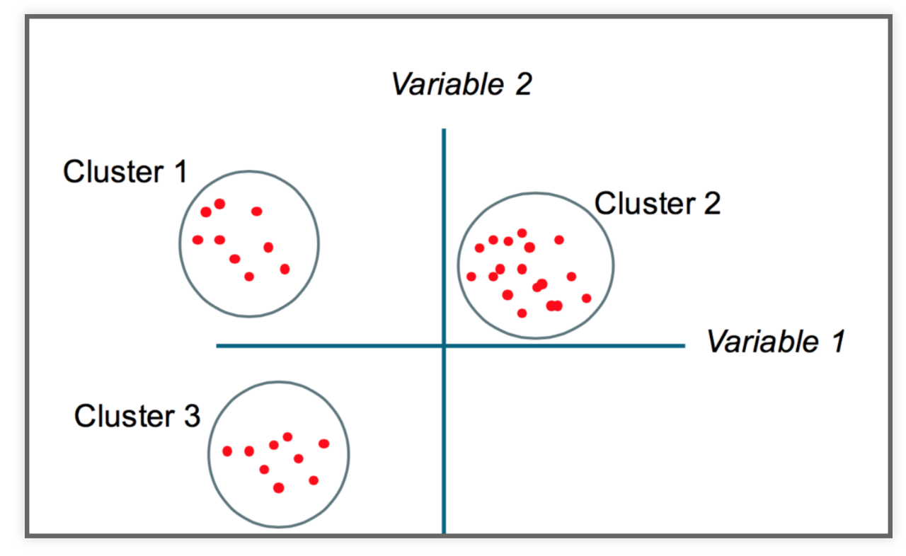
The goal
Partition a dataset into groups that have a similar set of attributes, or features, within the group and a dissimilar set of features between groups.
Minimize the intra-cluster variance and maximize the inter-cluster variance of features.
Some intuition
K-Means clustering
- Simple but robust clustering algorithm
- Widely used
- Important: user must specify the number of clusters
- Cannot be used to find density-based clusters
This is just one of several clustering methods
https://scikit-learn.org/stable/modules/clustering.html#overview-of-clustering-methods
A good introduction
How does it work?
Minimizes the intra-cluster variance: minimizes the sum of the squared distances between all points in a cluster and the cluster centroid
K-means in action

import altair as alt
from vega_datasets import data as vega_data
Read the data from a URL:
gapminder = pd.read_csv(vega_data.gapminder_health_income.url)
gapminder.head()
Plot it with altair
alt.Chart(gapminder).mark_circle().encode(
    alt.X("income:Q", scale=alt.Scale(type="log")),
    alt.Y("health:Q", scale=alt.Scale(zero=False)),
    size='population:Q',
    tooltip=list(gapminder.columns),
).interactive()
K-Means with scikit-learn
from sklearn.cluster import KMeans
Let's start with 5 clusters
kmeans = KMeans(n_clusters=5)
Lot's of optional parameters, but n_clusters is the most important:
kmeans
Let's fit just income first
Use the fit() function
kmeans.fit(gapminder[['income']])
Extract the cluster labels
Use the labels_ attribute
gapminder['label'] = kmeans.labels_
How big are our clusters?
gapminder.groupby('label').size()
Plot it again, coloring by our labels
alt.Chart(gapminder).mark_circle().encode(
    alt.X('income:Q', scale=alt.Scale(type='log')),
    alt.Y('health:Q', scale=alt.Scale(zero=False)),
    size='population:Q',
    color=alt.Color('label:N', scale=alt.Scale(scheme='dark2')),
    tooltip=list(gapminder.columns)
).interactive()
Calculate average income by group
gapminder.groupby("label")['income'].mean().sort_values()
Data is nicely partitioned into income levels
How about health, income, and population?
# Fit all three columns
kmeans.fit(gapminder[['income', 'health', 'population']])

# Extract the labels
gapminder['label'] = kmeans.labels_
Plot the new labels
alt.Chart(gapminder).mark_circle().encode(
    alt.X('income:Q', scale=alt.Scale(type='log')),
    alt.Y('health:Q', scale=alt.Scale(zero=False)),
    size='population:Q',
    color=alt.Color('label:N', scale=alt.Scale(scheme='dark2')),
    tooltip=list(gapminder.columns)
).interactive()
It....didn't work that well
What's wrong?
K-means is distance-based, but our features have wildly different distance scales
scikit-learn to the rescue: pre-processing
- Scikit-learn has a utility to normalize features with an average of zero and a variance of 1
- Use the
StandardScalerclass
from sklearn.preprocessing import StandardScaler
scaler = StandardScaler()
Use the fit_transform() function to scale your features
gapminder_scaled = scaler.fit_transform(gapminder[['income', 'health', 'population']])
Important: The fit_transform() function converts the DataFrame to a numpy array:
# fit_transform() converts the data into a numpy array
gapminder_scaled[:5]
# mean of zero
gapminder_scaled.mean(axis=0)
# variance of one
gapminder_scaled.std(axis=0)
Now fit the scaled features
# Perform the fit
kmeans.fit(gapminder_scaled)

# Extract the labels
gapminder['label'] = kmeans.labels_
alt.Chart(gapminder).mark_circle().encode(
    alt.X('income:Q', scale=alt.Scale(type='log')),
    alt.Y('health:Q', scale=alt.Scale(zero=False)),
    size='population:Q',
    color=alt.Color('label:N', scale=alt.Scale(scheme='dark2')),
    tooltip=list(gapminder.columns)
).interactive()
# Number of countries per cluster
gapminder.groupby("label").size()
# Average population per cluster
gapminder.groupby("label")['population'].mean().sort_values() / 1e6
# Average life expectancy per cluster
gapminder.groupby("label")['health'].mean().sort_values()
# Average income per cluster
gapminder.groupby("label")['income'].mean().sort_values() / 1e3
gapminder.loc[gapminder['label']==4]
gapminder.loc[gapminder['label']==2]